Performance Demonstration: Geodesic vs. Planar Distance

Context

A standard method of locating any point on Earth's surface is by using longitude (lon) and latitude (lat) coordinates within a particular spatial reference framework. The World Geodetic System 1984 (WGS84), identified by the code EPSG:4326 is the global standard used by the Global Positioning System (GPS). However, other regional frameworks exist such as the North American Datum (NAD83). This framework, identified as EPSG:4269 is the standard for spatial data across North America and is the coordinate system I explored in this experiment.

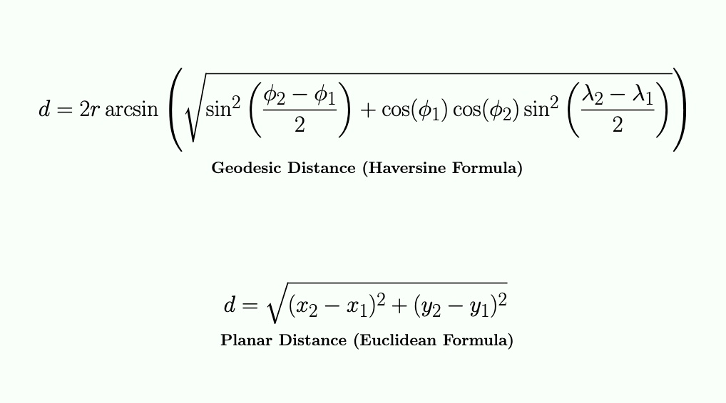
Assuming a spherical model for the Earth, calculating the distance between two points using their lon/lat coordinates can be accomplished with the Haversine formula, which involves relatively complex trigonometric functions to determine what is known as the Great Circle Arc, or Geodesic Distance. However, if we first project the Earth's spherical coordinates onto a 2D plane, we can simplify this task to use the Euclidean formula. This method is based on the Pythagorean Theorem to determine the Straight Line Distance between two points, known as Planar Distance.

While the geodesic approach is more accurate because it accounts for the curvature of the Earth, it is computationally more expensive for a program's runtime. My exp3-planar-vs-geodesic-distance-performance demonstrates this performance gap using real-world data obtained from the California (CA) Open Data portal. Specifically, it uses location data of CA power plants stored in a GeoJSON file under the EPSG:4269 (NAD83) spatial reference framework. Through this experiment, I also had the opportunity to get my feet wet with geoprocessing using Python 3 while extracting the necessary lat/lon information I needed from the dataset.

Implementation

The experiment begins with a Python 3 data preprocessing phase to extract lon/lat pair for each power plant's location. The original GeoJSON dataset from the CA Open Data portal was too small for meaningful benchmarking (less than 3k points), especially taking into account that some geospatial datasets can be massive in size and containing millions, if not billions, of points such as Light Detection and Ranging (LiDAR) datasets. Therefore, this phase scales the data into sets of 1k, 5k, and 10k points and adds synthetic noise to the last two sets to simulate a more realistic geographical distribution of coordinates.

The app relies on the structs GeoPoint and Point to handle geographic (pre-projected) and planar (projected) coordinate data, respectively. For the benchmarking process, it utilizes vector containers to manage these coordinate objects for batch processing.

To calculate planar distances, the app implements a Mercator Projection to map spherical coordinates, initially converted from degrees to radians, to a 2D Cartesian plane. While the longitude mapping is linear, the latitude mapping is non-linear and calculated using the logarithmic tangent of the adjusted latitude.

Edge case: The projection implementation clamps latitudes as a safeguard to the Mercator trigonometric function approaching infinity at the poles. This prevents the program crashing by limiting coordinates to the functional bounds of the projection ~ (+/- 85.05113).

The benchmarking process uses a simple timer utility (built around the C++ clock) to measure two distinct pipelines: a pairwise Haversine computation and a pairwise Euclidean (planar) computation. Each dataset is iterated 1,000 times to provide a better measurement window.

Example input:

# Each line contains a lon/lat pair separated by a comma

119.567892971,-36.137169611
-119.579712248,36.144318942
119.648391474,-36.2696401320001
-119.647437264,36.270308115
-119.128325036,36.2662977900001
# etc.

Results

For each dataset, the application reports in milliseconds the runtimes of performing both distance calculations: geodesic using the Haversine formula on lon/lat coordinates and planar using the Euclidean formula. It also reports the time difference between the two approaches showing the computational overhead of the more complex trigonometry as the data volume scales.

Example output:

----- Dataset: data/processed/points_1k.txt -----
Points: 1000
Geodesic (Haversine) time (1000 runs): 91 ms
Planar (Euclidean) time (1000 runs): 15 ms
Time difference: 76 ms


----- Dataset: data/processed/points_5k_noisy.txt -----
Points: 5000
Geodesic (Haversine) time (1000 runs): 461 ms
Planar (Euclidean) time (1000 runs): 76 ms
Time difference: 385 ms


----- Dataset: data/processed/points_10k_noisy.txt -----
Points: 10000
Geodesic (Haversine) time (1000 runs): 908 ms
Planar (Euclidean) time (1000 runs): 190 ms
Time difference: 718 ms

Testing

Unit tests using the GoogleTest framework validate the correctness of the Mercator projection and both distance functions. The test suites cover mathematical properties like symmetry and identity, along with edge cases such as latitude clamping near the poles and verifying that distances wrap correctly across the 180-degree Antemeridian (+179 to -179 longitude). The latter means that distances between points on opposite sides of the Antimeridian should be calculated across the shortest path rather than the "long way" around the globe.

Sample Haversine distance unit test

// Validate known distance: UC Riverside (UCR) to UC San Diego (UCSD)
// Coordinates from Google Maps, converted to ESPG:4269 NAD83 via epsg.io
TEST(HaversineDistanceTest, UCRToUCSD) {
  GeoPoint geo_p1{-117.328323, 33.9735855};  // UCR
  GeoPoint geo_p2{-117.2344872, 32.8810646};  // UCSD
  double dist = HaversineDistance(geo_p1, geo_p2);

  // About 90.5 mi = 145,645.6 meters using Google Maps
  // Haversine computes the great circle distance on a spherical Earth
  // Driving distance is longer due to winding streets
  // Haversine distance = ~ 121,800 meters
  EXPECT_GT(dist, 121000.0);
  EXPECT_LT(dist, 122000.0);
}

Sample projection unit test

// Latitude mapping is monotonic
TEST(ProjectionTest, LatitudeIsMonotonic) {
  // Keep lon constant to isolate lat behavior
  GeoPoint geo_p1{0, -20};
  GeoPoint geo_p2{0, 0};
  GeoPoint geo_p3{0, 20};
  GeoPoint geo_p4{0, 50};
  Point p_neg = GeoToPlanar(geo_p1);
  Point p_zero = GeoToPlanar(geo_p2);
  Point p_pos = GeoToPlanar(geo_p3);
  Point p_high = GeoToPlanar(geo_p4);

  // Increasing order should be conserved (including through zero)
  EXPECT_LT(p_neg.y, p_zero.y);
  EXPECT_LT(p_zero.y, p_pos.y);
  EXPECT_LT(p_pos.y, p_high.y);
}

Visual

Open in a new tab

Process Flowchart for Planar vs Geodesic Performance Demonstration

Discussion & Resources

As demonstrated by the experiment's output, by applying a Mercator projection, we can use simple Euclidean math instead of rather complex trigonometry, which significantly reduces CPU overhead as the data scales.

One limitation of this implementation is the accuracy tradeoff that comes with the faster performance. Projections simplify the distance calculation but they introduce geometric distortions in area, shape, distance, and/or direction, depending on which projection is used. However, because Earth's curvature can be seen as negligible over short distances, it can be mathematically treated as a flat plane when comparing two proximal locations. Therefore, the accuracy tradeoff can be considered insignificant for localized use cases such as calculation within a single city\s limits.

A compiler behavior I learned is Dead Code Elimination (DCE) such as for unused variables. I tracked the total distances for both the Haversine and Euclidean approaches, assigning them to dedicated variables for potential CLI output. However, since these totals are not currently used, a modern optimizer may identify the whole calculation loop as 'dead code' and skip it entirely. To prevent this, I used volatile sink variables to consume the unused ones. By qualifying these variables as volatile, we can force the compiler to treat the assignments as side effects that cannot be optimized away, to ensure the CPU performs every operation for the sake of an authentic benchmarking process.